The Mesh: The Beating Heart of the Finite Element Method
The main criteria for the preparation of each calculation model, always keeping in mind the metaphor “garbage in, garbage out”, lies in the structure’s discretization, also called mesh or calculation grid.
But what is a mesh? It is the set of primitive geometries (mono-bi-three dimensional), which allow to evaluate a structure passing from a continuous model (the reality) to a discretized model (finite elements), describing its physical-mathematical behavior through systems of partial differential equations, and reducing the latter to a system of algebraic equations.
The totality of these elements constitutes the discretized computational model and its “degrees of freedom”,i.e. all the possible variables generally calculated in the vertices of the elements, called nodes, which allow to evaluate how large the system of equations to be solved will be.
Geometries, Macro-categories and Calculation Models
The types of finite elements used in Kyma for the correct representation of a megayachts’ typical structures
(that will be detailed analyzed in the next in-depth study, the n.4) can be grouped into four macro-categories.
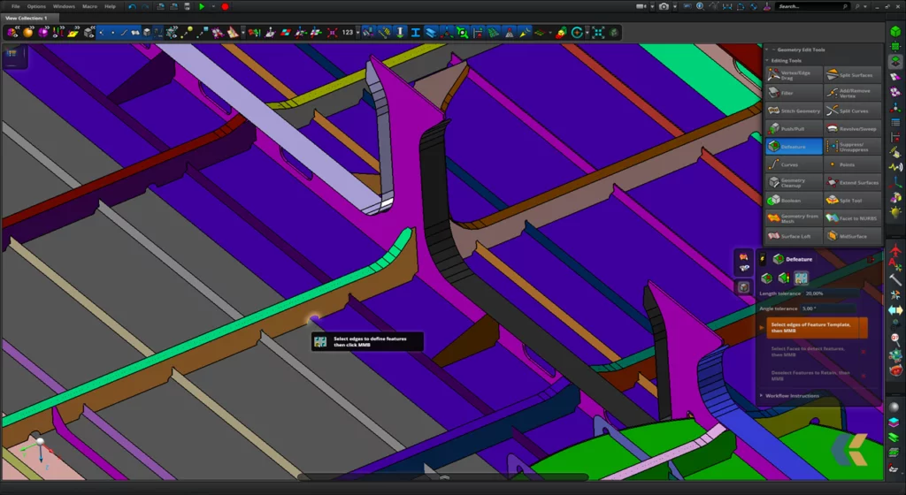
This simplification is useful to the FEM analyst because, also in the defeaturing’s calculation model preparatory phase, will be possible to decide the best physical-mathematical representation for each structure in order to obtain realistic results:
● Monodimensional Elements: they are mainly used for structures having a “main dimension”, generally the length, much bigger than the others (width and thickness). Depending on the type of analysis to be developed and the degree of precision of the results to be obtained, the internal library of MSC software allows the use of two, three or four-node one-dimensional elements. Each node has typically six degrees of freedom (three translations and three rotations).
● Bidimensional Elements: when the analysed structures have two main dimensions generally length and width, much bigger than the third (thickness), two different types of finite elements can be used, applying them both individually and simultaneously within the calculation model:
- Triangular Elements: thanks to their simplicity they historically represent the first type of bidimensional elements used. The internal software library allows the use of elements from three to thirteen nodes, whose choice is always linked to the type of analysis to be undertaken.
- Quadrangular Elements: evolution of triangular elements, are generally more reliable and precise. In this case four to sixteen nodes are available.
The bidimensional elements typically have five degrees of freedom per node and, if necessary, it’s possible request the software to use the sixth degree of freedom that represents the rotation in the plane of the element (drilling).
● Tridimensional Elements: when the structure has similar main dimensions, there is a need to represent its real geometry without anything to simplify. For this category of elements, that typically has three degrees of freedom per node, it’s possible use three different types of finite elements available in the library, applying them both individually and simultaneously within the calculation model:
- Tetrahedral Elements (four faces): as for triangular bidimensional elements, thanks to their simplicity represent the simplest finite element for a solid domain’s discretization. The internal software library allows the use of elements from four to sixteen nodes and the choice is always linked to the type of analysis undertaken.
- Hexahedral Elements (six faces): these are the most reliable tridimensional elements, and their use is always recommended, even in the preparatory phases of the calculation model. For this category is available a range of elements from eight to sixty-four nodes.
- Pyramidal Elements (five faces): similar to four faces’ elements, are generally used as a transition between tetrahedral and hexahedral elements. For this typology, elements between six and fifty-two nodes can be used.
When FEM analyst needs to use individually or simultaneously the above-mentioned categories of elements, respecting the “mesh congruence”, will be possible to choose wisely which types of finite elements to produce accurate results.
The choice will be based on the type of simulation to be developed, and the software library available which is associated with an internal mathematics for each element (linear, square elements, etc.).
In addition, each category of elements has several algorithms for generating the calculation grid, both automatic and manual, depending on the geometric complexity to be discretized. Also in this case, the preparatory phase of the calculation model gives fundamental results: a good designer must be able, possibly and compatibly with time and calculation resources, to generate “mappable” geometries, which can be discretized predominantly with quadrangular (in the case of surfaces) or hexahedral (in the case of solids).
Special elements: This category includes those elements whose internal mathematics help the FEM analyst in special situations, such as the coupling of non-uniform meshes, load or mass transfer, the assignment of boundary conditions etc. In Kyma the main special elements used are:
- R-type elements: in this subcategory of elements the most commonly used are RBE2 and RBE3;
- MPCs (Multi Point Constraints): typically used for setting linear contacts;
- Connector: mainly used for the union between structural parts, both welded and bolted.
The FEM Calculation Method among Pitfalls and Opportunities
The power of the Finite Element Method (FEM) consists in the simplification of the reality that surrounds us and its decomposition into small parts that allow to calculate the approximate solution (transition from continuous domain to discrete domain).
But this method hides some pitfalls: one of the main ones is the choice of mesh size to be used for the discretization of the structural model. In theory, and except in special cases, the smaller the calculation grid size, the more accurate and realistic the results will be.
In fact, the FEM analyst must always remember that the smaller the size of the finite elements used will result in higher number of degrees of freedom in the numerical model.
The direct consequence of this assumption is the computational cost, i.e. the time taken by the computer to solve the equations’ system that describe the computational model’s mathematics.
The Convergence Test and the Types of Meshing
According to the typologies and the geometries of the calculation model to be developed, in Kyma we define three macro-categories of meshing. The dimensions of these macro-categories are established on the mesh convergence test that must always be carried out in the preliminary phase to define the correct balance between results’ accuracy and time needed to solve the calculations.
There are three types of meshing:
- Coarse Mesh: mainly used for very large portions of yacht (eg: the hull girder’s assessment) and in the preliminary stages of development of the computational model, where is necessary to reduce as much as possible the computational effort. To achieve this type of calculation grid, the structure is stripped of almost all structural details.
- Standard Mesh: mainly used for the structural check (strength assessment) of small to medium-sized computational models (e.g. structural compartments), represents the right compromise between accuracy and calculation speed.
- Fine Mesh: used almost exclusively in detail models, can investigate with extreme precision any structural portions considered critical and potentially subject to breakage. Given the large number of finite elements necessary for the correct discretization of the geometries to be analyzed, in order not to generate very long computation times, it is used on small structural models or on particular areas of larger models (structural zoom) on which to investigate in more depth the response of the structure.
Mesh and Calculation Grid: Tools and Analysis for Realistic Results
The mesh’s construction for a computational model plays a main role to achieve realistic results, together with the preparatory defeaturing phase.
A good designer must be able, based on the type of calculation model to be developed and compatibly with the computational resources available, to establish:
- what is the type of finite elements that best represents the structure from a physical-mathematical point of view;
- the most correct calculation grid size to be applied to obtain correct results.
The analysis and the work’s organization followed in Kyma along the entire FEM calculation path allow to optimize every single step, expanding its radius and amplifying all its potential.